Excuse me, do you have time to talk about glue?

Dear reader – if you even exist and aren’t an ad-bot. I have been on an over long sick leave. That’s the reason why I haven’t published any new posts, especially almost right away after the start. So this is not the typical “Hey I have a blog, please check this out!!1” and after a couple of posts and hardly any visitors: “but it’s so hard to publish new stuff and all this actually takes a lot of time, so let’s just let the time fade all this away” -explanation.. Well, readers or no, I think it’s good to at least to try to tell what I do and how and why – in an understandable and dense way. These are challenges, so training is for good. And sharing is caring: At least I have gotten ideas from conferenses, scientific articles and just googling things.. #paybacktime

What could be a better motivator to publish a new post than money? Many other, to be honest. But I just paid an extra year for this domain so publishing gives some instant value for the “investment”. One more specific reason could be a colleague who asked me if I still have my GLUE thing. Yes I have, but like too many times before, it was not documented properly. If at all. I know especially now that documenting (and having a specific place for them) is vital if the purpose is to use them later. A blog then? 🙂 I haven’t been doing anything hydraulic modelling related lately, so please let me tell something old stuff while updating the laptop, getting  familiar with the keyboard and working routines and remembering too many forgotten passwords.. I suppose I never emphasized properly (or enough) why GLUE method is so good. I still think it’s a very good way to make your modelling and results even better. I’ll use my old “Ice-GLUE” as an example. I wrote another post about this some time ago.

I don’t know if I ever realized GLUE (generalised likelihood uncertainty estiation) method correctly and there is still plenty to learn for sure, but I became a fan of it already when I did my master thesis. Not applying the method then as the plan for the thesis was already made, but it would definitely have been a great help and make the results even better (well it was good enough if you ask reviewers and the 2008 version of me 🙂 Link to the abstract of the master thesis). I have this book about GLUE and I can recommend it if you want to learn more – and numerous scientific articles. At least I’m not the only one liking it.

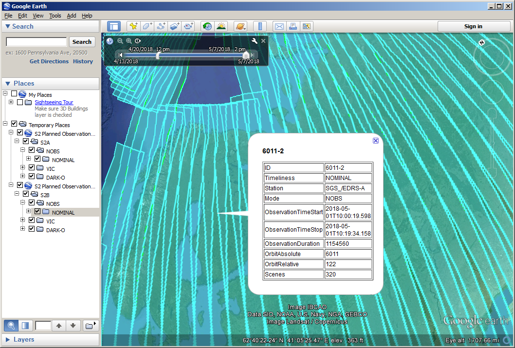
So how does my version of GLUE and the first ever (and still the best) hydraulic model for me, HEC-RAS, work together then? I personally named that as GLUE-RAS..

  1. You don’t have to have a fully calibrated hydraulic river model. But unfortunately, as this isn’t a miracle doing everything for the user, it should be measured well and be able to produce good results. As the values can and will for example change with the decreasing and increasing discharge, downstream water elevation and growing and diminishing roughness factors (aquatic plants, landslides to river etc.) so it’s luckily useless to try to be perfect here. Pay attention observations and measurements have a good quality. Always.
  2. Try to think what kind of ranges the most important and/or meaningful physical quantities can have. In this current version you must give a minimum and a maximum value. Try to be realistic, remembering that the world can give surprises too. In a river and in a real life.. For a river with ice jam possibilities I thought these are important:
    • Manning n values for the channel and left and right over banks (LOB, ROB). I see I had added an option to use the actual Manning n values or then a partition or multiplier of the original geometry n-values. I have never used that, though.
    • Ice thickness. Meaning the thickness of ice before any ice jams. In here you can have only one ice thickness for the whole river, but that value can be extended to overbanks or then they are zero.
    • Ice cover Manning values. What is the roughness of the ice cover? Again, like with ice thickness the same value is applied overall the river.
    • Ice friction angle
    • Ice porosity
    • Ice stress K1 ratio
    • The maximum underice velocity
    • If there is an ice jam, what the manning n value of it?
    • What is the range of the discharge coming in into the river? Only one channel to have an input discharge. A good programmer could extend this to multiple incoming flows
    • What is the range of water elevation at the downstream of the model? This tool only have one place to where all the water in the model flows to.
    • The lowest cross section of the ice jam.
    • The length of the ice jam.
      Naturally or surprisingly these are the things you can change/modify when doing your model geometry too.
  3. How many plans you want to make? Keep in mind there can be 1-99 calculations per one HEC-RAS plan..
  4. Number of decimals. Is almost always not more than 3, but for some reason I allowed something else too. I haven’t tried this.
  5. Number of projects. A normal full HEC-RAS project has got 99 plans, so 10 full projects is almost 1000 results. Take care of hard disk space and time you are allowed to use..
This is how the Excel file looks like.

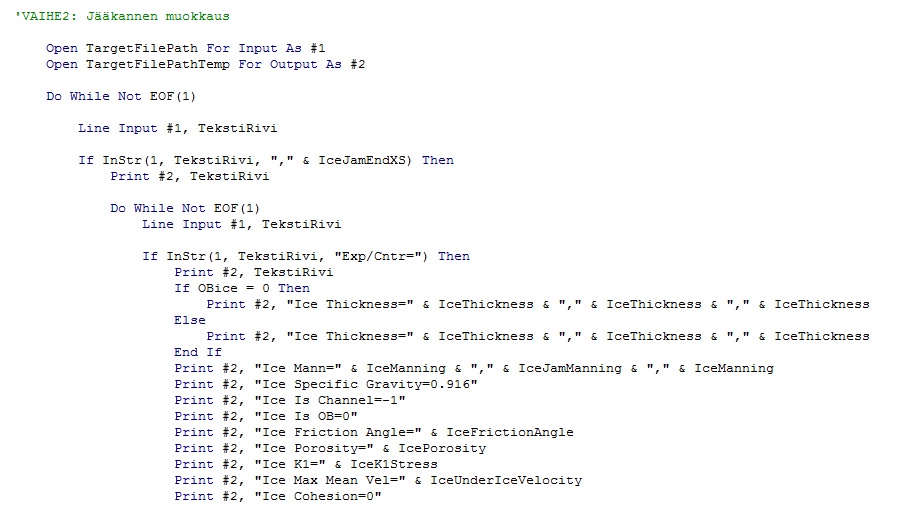
So what does this do then? Basically this is like a random number generator, taking those before mentioned quantities and giving them new values from the given range. I used Excel and its VBA (Visual Basic for Application) programming language. In short, it generates numerous HEC-RAS project plans differing a bit from each other but which still are inside the range you just have defined in the Excel form. Please check out this book too for “real” way to break the HEC-RAS code. I just didn’t get everything working – and it’s not book’s and model’s fault.

And this is a where the (amateur) magic happens..

Maybe one possibility to make an improvement could be to give a user a possibility to use some kind of distribution (like normal distribution?) instead the basic uniform distribution. Another improvement could be to define which one of these are going to randomised and which one not. Well, if you now give the same mimimum and maximum value, it should always generate a one and wanted value as a “random” value.

To be honest, I have never tried the flow change location. Or at least I don’t remember it (that can happen). For some reason I added that fuction anyway. Maybe if there are river junctions and the discharge is divided – but you don’t have the geometry of the whole river for example.. You could give a location and the amount of percentage of the discharge to get removed from the model?

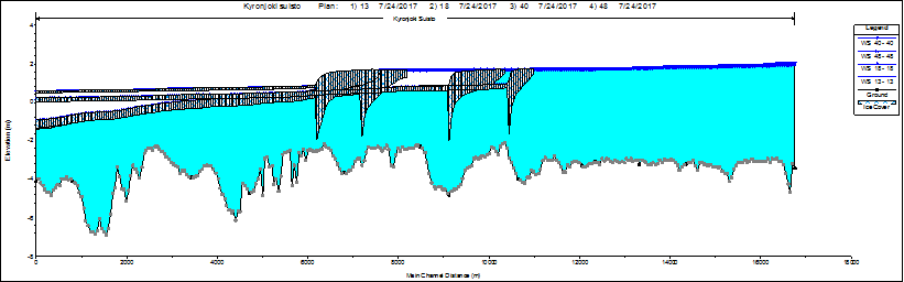
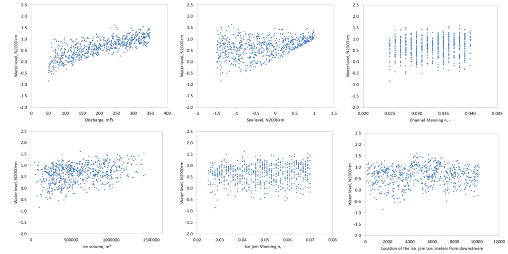
Then you just run the large amount of HEC-RAS projects and get the results. You get lots of result files. A good programmer would automatize this more to get the results automatically to Excel, but I’m not a good one 🙂 Anyway, having these point clouds you might get a better idea or proofs that some things you have defined (discharge, downstream water elevation, ice jam location, amount of ice etc.) in the area are really meaningful or some are totally meaningless. Or things you thought are meaningless are still meaningful if other things and stars have the right value or position.

I have used this image before too. Sorry! But this is how the results look like. You can or cannot see the meaning of life from these? 😉

A good text always summarizes the key point.. Err.. Well a note to self says anyway:

  • Document what you do, as you or somebody else might need the information later..
  • Hello internet! I’m (trying to be) back.
  • I noticed there is one draft (in Finnish) from the past in this blog when I finally got logged in, so stay tuned – I try to be a bit quicker (don’t count your chickens before they hatch though, Juha)
  • As the computation efficiency of the modern computers is so good, I really wonder what is the reason to not use this kind of method in problem solving
  • Knowing uncertainty can eventually bring more certainty?


Satelliittikuvien hyödyntäminen virtausmallinnuksessa

English summary and a wrap-up for busy TL;DR people: This post is about calibrating a hydraulic model with remote sensing imagery. Remote sensing is a great help, but does not replace traditional, continuous and reliable hydrological observations. The example is from Lake Kuortaneenjärvi and Lapuanjoki River area and based on April 2018 flood. 

Tulvakartan laatiminen järvelle on melko yksinkertaista. Määritetystä vedenpinnan korkeudesta vähennetään maanpinnan korkeus, jolloin tuloksena saadaan vesisyvyys eri kohdissa. Jos ja kun järvi laskee jokeen, ei vakavesikarttaa voi kuitenkaan jatkaa loputtomiin alavirtaan joen kaltevan vesiprofiilin vuoksi. Kaltevuus riippuu mm. joen pohjan pituuskaltevuudesta tai vesitilanteen mukaan muuttuvista virtaamasta, joen alajuoksun vedenkorkeudesta tai vaikka jääpadoista. Virtavesien vedenkorkeuksia voidaan selvittää virtausmallin avulla, jossa uoma on yksinkertaisimmillaan esitetty virtaussuuntaan nähden kohtisuorasti olevien poikkileikkauksien avulla. Vesi ylimmästä poikkarista sisään ja alimmasta ulos, jos oikaisaan ja yritettään päästä hiljalleen asiaan 🙂

Juts another nice image to catch your attention 😉

Virtausmallin laskemien vedenkorkeuksien tarkistamiseen tarvitaan havaintoja. Vaikka vedenkorkeuden havaintoverkko kattaa noin 870 asemaa, ei havaintoasemia satu kovin tiheästi saman vesistön varrelle. Ja kun virtausmalliin joutuu monesti kiinnittämään yhden vedenkorkeusaseman alapuoliseksi reunaehdoksi, ei varsinaiseen mallinnettavaan alueeseen välttämättä enää olekaan havaintoja. Toinen havaintoihin liittyvä haaste on se, että suurin osa havainnoista edustaa normaalia vesitilannetta. Pelkkien uomassa pysyvien vedenkorkeuksien mukaan kalibrointi ei kovin varmaa perustaa anna uomasta leviävien tulvien todenmukaiseen toistamiseen. Vähän kuin opettelisi ajamaan pikkuautoa ja lähtisi niillä opeilla täysperävaunun rattiin.

Joen vedenpinta poikkileikkauksessa ennen tulvaa ja tulvan aikana.

Mistä lisää havaintoja? Tässä kohtaa kentällä tehtävät yksittäisetkin tulvahavainnot ovat tärkeitä. Kiitos kaikille työn, mielenkiinnon ja vapaaehtoisuuden puitteissa havaintoja tekeville! Toinen lähde on kaukokartoitus. Netissä on useita paikkoja, joissa voi kuka tahansa katsella satelliittien napsimia kuvia ja värittää niitä eri filttereillä. Sentinel Hubista löytyy Playground ja EO Browser, joista löytyy tällä hetkellä hyödyllisimmäksi todetun Sentinel-2 -satelliitin kuvia.

EO Browser

Pilvettömältä taivaalta otettu kuva näyttää NDWI-filtterillä (Normalized Difference Water Index) kivasti vesialueet. Toki silmä pitää pitää kädessä, sillä esim. pilvien varjot ja näin keväällä lumi voivat värjäytyä sinisävyiseksi. Samoin tulvan peittämän ja ihan vaan kostean, tumman maanpinnan  ero voi olla häilyvä ja vihreän kasvillisuuden seassa oleva tulva voi olla vaikea tulkita. Vaikka optinen satelliitti kuvaisi kuinka monella kanavalla, muodostaa pilvi aina jonkinlaisen häiriön kameran ja maanpinnan väliin. Eli kun satelliitti joskus sattuu ylittämään mielenkiinnon kohteena olevan alueen, pitää toivoa että sää on kirkas. Näiden pitäisi sitten vielä natsata vesistön tulvahuipun kanssa.. Sentinelin tulevat ylilentoajat saa muuten Euroopan avaruusjärjestö ESAn sivuilta esim. Google Earthiin avautuvana .kml-tiedostona.

Sentinel-satelliitin ylilentojat Google Earthissa

Muutama vuosi sitten tuli tehtyä SYKEn Vesistömallijärjestelmää varten pientä virtausmallipohjaista tarkistusta Kuortaneenjärven purkautumiskäyrästä (eli mikä on järven luusuan virtaama eri vedenkorkeuksilla). Tätä varten Etelä-Pohjanmaan ELY-keskus mittasi poikkileikkauksia, joista laadin HEC-RAS-mallin ja mallinsin purkautumiskäyriä sekä nykytilanteelle että muutamille perkaus- ja patomuokkausvaihtoehdolle. Havaintojen puolesta tämä on siitä hyvä kohde, että itse järven vedenkorkeuden seurannan lisäksi hieman Lapuanjokea alaspäin löytyy Karan sillan havaintoasema. Kun Karan sillan vedenkorkeushavaintoja ja niistä johdettua virtaamaa käyttää mallin lähtötietoina, voi ylimmän poikkileikkauksen mallinnettuja vedenkorkeuksia vielä verrata Kuortaneenjärven havaintoihin. Mallinnettavalta alueelta voi sitten vaikka toivoa sopivaa optista satelliittikuvaa täydentämään havaintoja.

..ja varmaan arvasittekin että sellainenhan löytyi kun tätä juttua on jo näin pitkälle pohjustettu 🙂 Tallensin Sentinel Hubista 21.4. tilanteen kuvana ja väänsin sen itse koordinaatistoon. Sitten mallinsin kuluvan huhtikuun tapahtumat yhdellä muuttuvan virtauksen mallinnuksella. Poikkeuttamalla jo aiemmin ihan realistisia arvoja sisältäneitä, uoman ja tulva-alueen pinnan  karkeutta kuvaavia Manningin kertoimia mallinnettu ja havaittu tulva-alue napsahtivat ihan kohtuullisesti kohdalleen.

21.4.2018 otetusta Sentinel-2 NDWI-värjätystä kuvasta tulkitun tulva-alueen (sininen) ja HEC-RAS-mallinnuksen (punainen) vertailua.

Myös Kuortaneenjärven mallinnettu ja havaittu pinta seurailevat kivasti toisiaan, poislukien pieni sekoilu tulvan alkaessa, mutta tämä selittynee tarkistamattomien virtaama-arvojen käytöllä. Virtaama tuskin  laski  14.-18.4. jaksolla, mutta tuon jälkeen palattiin taas nousu-uralle.

Kuortaneenjärven havaittujen ja laskettujen vedenkorkeuksien vertailua

Hyvä kirjoitus pyrkii aina poimimaan jonkun pointin alustuksesta ja vetämään tekstin yhteen. Hoidan poiminnan animoituna giffinä, josta näkyy miten tuo joen vedenpinnan profiili on jopa heti järven jälkeen kalteva. Hieman, mutta kuitenkin:

Kuortaneenjärven luusuan ja Lapuanjoen alun pituusprofiili huhtikuussa 2018

Ja summaus: Satelliittikuva toi varmuutta virtausmallin antamiin tuloksiin ja tällä parametrisetillä uskaltaisi jo huomattavasti varmemmin lähteä mallintamaan harvinaisia, keskimäärin 50 tai 100 vuoden välein esiintyviä tulvia. Virtausmallintajana en lähtisi korvaamaan perinteistä havaintoverkkoa kaukokartoituksella vaan täydentämään. Satelliittikuvista ei saa pitkää aikasarjaa esim. toistuvuusanalyysia varten, mutta tietyn ajanhetken pistemäisen havainnon se täydentää hienosti laaja-alaiseksi tilannekuvaksi. Näissä hommissa tietoa on vielä harvoin liikaa.

Linkkivinkkejä:


Espoon Kirkkojärven kevyen liikenteen väylän korotus

Espoon Kirkkojärvellä on vesi edelleen korkealla ja Twitterissä tuli vastaan havainnollistava video, jossa kevyen liikenteen väylä oli poikki ja ehdotettiin väylän korotusta, jolloin se voisi toimia myös tulvavallina.

Tein aiemmin tulvahuipun aikaan alueesta virtausmallin. Tuolloin sille ei ollut sen kummempaa käyttöä kuin todeta, että malli toisti kohtuullisesti alueella olevan tulvan. Myöhemmin sillä tuotettiin Vesistömallijärjestelmään Kirkkojärven alueen vedenkorkeus-tilavuus-käyrät. Virtausmalli on laadittu HEC-RAS-ohjelman 2D-mallilla, jonka avulla on todella helppoa ja nopeaa tuottaa näyttävän näköisiä tuloksia. Tällöin on entistä tärkeämpää ymmärtää katsoa tulosten taakse ja Kirkkojärvenkin kohdalla todeta/paljastaa, että mallista mm. puuttuu todellinen Espoonjoen uoma (askartelin Maanmittauslaitoksen km2-korkeusmalliin käsipelillä 1,5-2 metrin syvyisen kapean ojan), jo 9 vuotta vanhasta korkeusmallista puuttuu mm. Kirkkojärven koulu ja virtaamahavainnotkin ovat ymmärtääkseni epävarmoja. Tulokset kuitenkin vastasivat kohtalaisella tasolla alueelta otettuja tulvavalokuvia.

Tietämättä sen enempää mitä toimenpiteitä Kirkkojärvellä on meneillään, päätin käyttää lounastauon puistokäytävän vaikutusten selvittämiseen. Tielinjan korotus on helppoa, jos malliin on alun alkaen viety avoimen Digiroad -aineiston teiden keskilinjat. Valmiiksi löytyvää tielinjaa voi korottaa esim. pato/pengertoiminnon avulla.

Kirkkojärven puistokäytävän korotus. Harmaa täyttä on korotusta, harmaa viiva alkuperäinen korkeus. Kirkkokatu kuvassa oikealla.

Kun tietä korottaa tarpeeksi, on tietysti selvää ettei vesi enää mene sen yli. Mallilla tuli kuitenkin myös selvitettyä, ettei tulva-alueen pienentäminen tietä korottamalla muuta jäljelle jäävän tulva-alueen vedenkorkeuksia. Ei ainakaan niin, että tulva-alue juuri muuttuisi. Vedenkorkeuden muutokset pyörivät sentin tasolla, mikä lähtötietojen epävarmuudet huomioiden on merkityksetöntä. Isompaa muutosta taisi tulla sillä, että ao. gif-kuvan  tulva-alueiden syvyyksien värimääritykset eivät menneet ennen-jälkeen -kuvissa yksiin 🙂

Consideration of river ice breakup uncertainties in HEC-RAS

(Update on 2/1/2018:  I finally decided to finish and publish this private blog post about handling the uncertainties in the ice jam modelling of HEC-RAS software. The reason to do this on a holiday day is a new HEC-RAS River Ice Modeling forum, which was just founded on the already excellent HEC-RAS help forum.)

This has nothing to do with rive ice breakup, it’s just a too nice photo to ignore 🙂

River ice breakup jams may cause significantly high water elevations. In some regions they may be the only source of floods in terms of flooding outside the river banks.  If it is challenging to obtain all the information for  an open water flood (i.e. without ice), it surely is the case with river ice. In addition to the basic data (discharge, downstream water elevation, Manning’s roughness coefficients) river ice simulations in HEC-RAS require for example the following information:

  • the location of the ice jam toe
  • ice jam and solid ice cover roughness (Manning’s n)
  • cross section range where the ice jam is allowed to form up
  • several ice jam parameters like porosity, maximum under ice velocity, friction angle, K1 stress ratio etc.

Now, a very good question is, that are you in the first place able simulate a single “representative” ice jam scenario by just locking the parameters with single and default values? By doing so at least I, as a modeller, would be really hesitant to give the customer a reliable estimation about the ice jam probability or the damage potential of the ice jam flood. As each winter and ice breakup event will have a different discharge, ice jam formation location, downstream water elevation and ice volume contributing the ice jam, it would be quite dangerous to lock yourself up with a single parameter set. Neither can we be sure about the correctness about the model’s default values for the ice cover parameters. And it is always a good practice to clarify the uncertainties in your modelling project anyway.

..especially when there is a way to do this efficiently in HEC-RAS! You can use VBA code to change the HEC-RAS parameters. This can be done by using the HECRASController API or semi-automatically to modify the source HEC-RAS files (geometry file, boundary condition file and simulation plan file). I did the latter with VBA – as I couldn’t figure out how to manage the varying location of the ice jam toe and allowed ice jam length. The results were however dug out of the hundreds of simulations by the help of Chris Goodell‘s amazing book, where the usage of HECRASController is covered in detail.

The basic idea is to define each parameter a typical range, generate hundreds of parameter combinations and then perform the simulations and  analyse the results. It is unnecessary to mention, that local knowledge and observations are a crucial help in this work. The amount of data is huge in this method, but with some automation it will not take much more time compared to old fashioned single-parameter-modelling. As a result you will get a more confident picture about the significance of each parameter. Some parameters are of course obvious (like the amount of ice in the ice jam), but the ice jam location, downstream water elevation and discharge may cause varying effects thorough the river reach. Further work is still needed for example in handling the joint probability of discharge and sea water level.

For example in a river profile picture below you can see how the same flood water elevation in the upstream may be achieved with very different sea level elevations, ice jam locations and ice volumes. Discharge can’t be seen on these profiles, but that varied a lot as well.

Results may be also taken into a more abstract level like “point clouds” below. I got a lot of inspiration for these point cloud figures from professor Keith Beven’s generalized likelihood uncertainty estimation (GLUE) papers. I can highly recommend his books and papers around uncertainty estimation. Each little picture below contains the same amount of water elevations (n=936) but they are presented against different parameter or boundary condition.

This HEC-RAS method has been applied for four Finnish rivers when it comes to ice jams. As the method is of course capable of simulating the corresponding open water situation, you can use this to obtain rating curves for lake outlets without any real or insufficient observations. But back to floods: Water elevations can be further refined into flood inundation maps, where the parameter uncertainty is taken into account. An example of this is presented below:

I presented a project covering this method in the 19th CRIPE workshop in Whitehorse, Canada. I think I have never been so nervous to give a presentation as the quality of the workshop was so high and there were the best river ice experts and gurus in the audience. I was glad (and relieved) to receive positive feedback and people encouraged me to continue with this topic. I highly recommend the CRIPE workshops for anyone interested in river ice research. There were not too many of us from Europe.

The project by the way is a joint project between Finnish Environment Institute and  Centre for Economic Development, Transport and the Environment for South Ostrobothnia. The river ice breakup modelling is a part of a larger entity around developing the estuary of River Kyrönjoki. There is a great blog post (in Finnish) about the entity in here. At the moment we have done the simulations for the current river bed and identified some interesting locations to where some modifications will be applied. We will apply the model geometry and run the same simulations again and see if the alterations have any significant and cost-effective benefits.

Below is my CRIPE 2017 presentation about river ice breakup modelling and how we took the uncertainties account:


We also wrote a conference paper about this. A direct link to our paper is here and the complete proceedings of the workshop can be found here.

Do you have any questions, comments or suggestions for this topic? Have your say in the comments below, please!